Superset and Jupyter notebooks on AWS as Service

Jupyter Notebook (In EC2 Instance):

The following script is written to run jupyter notebook as a server inside the AWS EC2 instance which you can access from your desktop/laptop if EC2 instance is accessible from your machine:

• $ conda activate python37
• $ jupyter notebook –generate-config
  • This will create the jupyter_notebook_config.py configuration file inside your working folder i.e. /home/<username>/.jupyter/
• $ jupyter notebook password  
  • You can set the password here
• $ vi /home/centos/.jupyter/jupyter_notebook_config.py
  • Edit the following 2 lines 
  •   c.NotebookApp.ip = ‘0.0.0.0’
  •   c.NotebookApp.port = 8888
• $ jupyter notebook

Apache Superset (In EC2 Instance):

• Install
  • $ pip install superset 
  • Installing Apache Superset into CentOS 7 with Python 3.7
• Run:
  • $ superset run -h 0.0.0.0 -p 8080 –with-threads –reload –debugger

That’s all.

@avkashchauhan

Installing Apache Superset into CentOS 7 with Python 3.7

Following are the starter commands to install superset:

• $ python –version
  • Python 3.7.5
• $ pip install superset

Possible Errors:

You might be hitting any or all of the following error(s):

Running setup.py install for python-geohash … error
ERROR: Command errored out with exit status 1:

building ‘_geohash’ extension
……
unable to execute ‘gcc’: No such file or directory
error: command ‘gcc’ failed with exit status 1

gcc: error trying to exec ‘cc1plus’: execvp: No such file or directory
error: command ‘gcc’ failed with exit status 1

Look for:

• $ gcc –version <= You must have gcc installed
• $ locate cc1plus <= You must have cc1plus install

Install the required libraries and tools:

If any of the above components are missing, you need to install a few required libraries:

• $ sudo yum install mlocate <= For locate command
• $ sudo updatedb  <= Update for mlocate
• $ sudo yum install gcc <=For gcc if you don’t have
• $ sudo yum install gcc-c++  <== For cc1plus if you dont have

Verify the following again:

• $ gcc –version
• $ locate cc1plus
  • /usr/libexec/gcc/x86_64-redhat-linux/4.8.2/cc1plus

Note:

• If you could locate cc1plus properly however still getting the error, try the following
  • sudo ln -s /usr/libexec/gcc/x86_64-redhat-linux/4.8.2/cc1plus /usr/local/bin/
• Try installing again

Final Installation:

Now you can install  superset as below:

• $ pip install superset
  • Python 3.7.5
    Flask 1.1.1
    Werkzeug 0.16.0
• $ superset db upgrade
• $ export FLASK_APP=superset
• $ flask fab create-admin
  • Recognized Database Authentications.
    Admin User admin created.
• $ superset init
• $ superset run -p 8080 –with-threads –reload –debugger

 

That’s all.

@avkashchauhan

Conda Python 3.5 and OpenCV 3 with Matplotlib and QT5 backend

As title suggests lets get to work:

Create the Conda Environment with Python 3.5

$ conda create -n python35 python=35
$ conda activate python35

Inside the conda environment we need to install pyqt5, pyside, pyobj-core, pyobjc-framework-cocoa packages:

Installing QT5 required packages inside Conda:

$ conda install -c dsdale24 pyqt5
$ conda install -c conda-forge pyside
## Note: I couldn;t find these with conda on conda-forge so used pip
$ pip install pyobjc-core
$ pip install pyobjc-framework-cocoa

Verifying Python 3.5:

$ python

Python 3.5.4 |Anaconda, Inc.| (default, Feb 19 2018, 11:51:41)
[GCC 4.2.1 Compatible Clang 4.0.1 (tags/RELEASE_401/final)] on darwin
Type "help", "copyright", "credits" or "license" for more information.
>>>

Checking backend used by matplotlib:

import matplotlib
matplotlib.get_backend()

If you see ‘MacOSX‘ means it is using MacOSX backend and we need to change it to qt as below:

Changing matplotlib backend to use QT5:

matplotlib.use('qt5agg')
matplotlib.get_backend()

This will result as qt5agg backend to be used with CV2.

Sample code to show image using OpenCV3

Trying a sample OpenCV3 code to show image:

import cv2
image = cv2.imread("/work/src/github/aiprojects/avkash_cv/matrix.png")
import matplotlib.pyplot as plt
plt.figure()
plt.imshow(image)
plt.show()

This is how image rendered with QT5 backend:

That’s it, enjoy!!

@avkashchauhan

 

 

 

 

 

 

Compile OpenCV3 with Python3.5 Conda environment on OSX Sierra

As title suggests, lets get is going…

Create the Conda Environment with Python 3.5

$ conda create -n python35 python=35
$ conda activate python35

Verify the Conda Environment with python 3.5

$ python 
Python 2.7.14 |Anaconda custom (64-bit)| (default, Dec 7 2017, 11:07:58)

Now we will install tensorflow latest which will install lots of required dependency I really needed:

$ conda install -c conda-forge tensorflow

Python run time environment and Folder

Now we will look to confirm the python path

$ which python
/Users/avkashchauhan/anaconda3/bin/python

Now we need to find out where the Python.h header file is which will be used as the values for PYTHON3_INCLUDE_DIR later:

$ ll /Users/avkashchauhan/anaconda3/envs/python35/include/python3.5m/Python.h

Now we need to find out where the libpython3.5m.dylib library file is which will be used as the values forPYTHON3_LIBRARY later:

$ ll /Users/avkashchauhan/anaconda3/envs/python35/lib/libpython3.5m.dylib

Lets clone the OpenCV master repo and opencv_contrib at the same base folder and as below:

$ git clone https://github.com/opencv/opencv
$ git clone https://github.com/opencv/opencv_contrib

Lets create the build environment:

$ cd opencv
$ mkdir build
$ cd build

Now Lets configure the build environment first:

$ cmake -D CMAKE_BUILD_TYPE=RELEASE \
 -D CMAKE_INSTALL_PREFIX=/usr/local \
 -D OPENCV_EXTRA_MODULES_PATH=../../opencv_contrib/modules \
 -D PYTHON3_LIBRARY=/Users/avkashchauhan/anaconda3/envs/python35/lib/libpython3.5m.dylib \
 -D PYTHON3_INCLUDE_DIR=/Users/avkashchauhan/anaconda3/envs/python35/include/python3.5m/ \
 -D PYTHON3_EXECUTABLE=/Users/avkashchauhan/anaconda3/envs/python35/bin/python \
 -D BUILD_opencv_python2=OFF \
 -D BUILD_opencv_python3=ON \
 -D INSTALL_PYTHON_EXAMPLES=ON \
 -D INSTALL_C_EXAMPLES=OFF \
 -D BUILD_EXAMPLES=ON ..

The configuration shows following key settings:

......
......
-- Found PythonInterp: /Users/avkashchauhan/anaconda3/bin/python2.7 (found suitable version "2.7.14", minimum required is "2.7")
-- Could NOT find PythonLibs: Found unsuitable version "2.7.10", but required is exact version "2.7.14" (found /usr/lib/libpython2.7.dylib)
-- Found PythonInterp: /Users/avkashchauhan/anaconda3/envs/python35/bin/python (found suitable version "3.5.4", minimum required is "3.4")
-- Found PythonLibs: YYY (Required is exact version "3.5.4")
....
-- Python 3:
-- Interpreter: /Users/avkashchauhan/anaconda3/envs/python35/bin/python (ver 3.5.4)
-- Libraries: YYY
-- numpy: /Users/avkashchauhan/anaconda3/envs/python35/lib/python3.5/site-packages/numpy/core/include (ver 1.12.1)
-- packages path: lib/python3.5/site-packages
--
-- Python (for build): /Users/avkashchauhan/anaconda3/bin/python2.7
-- Pylint: /Users/avkashchauhan/anaconda3/bin/pylint (ver: 1.8.2, checks: 116)
--
General configuration for OpenCV 3.4.1-dev =====================================
-- Version control: 3.4.1-26-g667f5b655

Building the OpenCV code:

Now lets build the code:

$ make -j4

The successful build output end with the following console log:

Scanning dependencies of target example_face_facemark_demo_aam
[ 99%] Building CXX object modules/face/CMakeFiles/example_face_facemark_demo_aam.dir/samples/facemark_demo_aam.cpp.o
[ 99%] Linking CXX executable ../../bin/example_face_facemark_lbf_fitting
[ 99%] Built target example_face_facemark_lbf_fitting
[ 99%] Building CXX object modules/face/CMakeFiles/opencv_test_face.dir/test/test_facemark_lbf.cpp.o
[ 99%] Linking CXX executable ../../bin/example_face_facerec_save_load
[ 99%] Built target example_face_facerec_save_load
[ 99%] Building CXX object modules/face/CMakeFiles/opencv_test_face.dir/test/test_loadsave.cpp.o
[100%] Building CXX object modules/face/CMakeFiles/opencv_test_face.dir/test/test_main.cpp.o
[100%] Linking CXX executable ../../bin/example_face_facemark_demo_aam
[100%] Built target example_face_facemark_demo_aam
[100%] Linking CXX executable ../../bin/opencv_test_face
[100%] Built target opencv_test_face

Lets install is locally:

To install the final library try the following:

$ sudo make install

Once install is completed you will confirm the build output as below:

$ ll /usr/local/lib/python3.5/site-packages/cv2.cpython-35m-darwin.so

Copying final openCV library to Python 3.5 site package:

As we know that Python 3.5 Conda environment folder site-packages is here:

/Users/avkashchauhan/anaconda3/envs/python35/lib/python3.5/site-packages

So we will copy to final cv2.cpython-35m-darwin.so to Python 3.5 Conda environment folder site-packages as cv2.so as below:

$ cp /usr/local/lib/python3.5/site-packages/cv2.cpython-35m-darwin.so 
     /Users/avkashchauhan/anaconda3/envs/python35/lib/python3.5/site-packages/cv2.so

Confirm it:

$ ll /Users/avkashchauhan/anaconda3/envs/python35/lib/python3.5/site-packages/cv2.so

Verification OpenCV with Python 3.5:

Now Verify the OpenCV with Python 3.5 on Conda Environment:

$ python 
Python 3.5.4 |Anaconda, Inc.| (default, Feb 19 2018, 11:51:41)
[GCC 4.2.1 Compatible Clang 4.0.1 (tags/RELEASE_401/final)] on darwin
Type "help", "copyright", "credits" or "license" for more information.
>>> import cv2
>>> cv2.__version__
'3.4.1-dev'
>>>

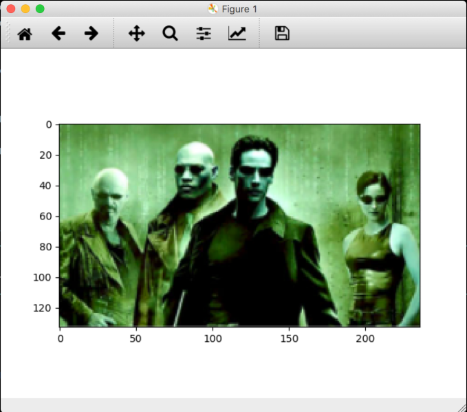
Now lets run OpenCV with as example:

import numpy as np
import cv2

# Load an color image in grayscale
img = cv2.imread('/work/src/github/aiprojects/avkash_cv/test_image.png', 0)
while(True): 
    cv2.startWindowThread() 
    cv2.namedWindow("preview")
    # Display the resulting frame 
    cv2.imshow("preview", img) 
    if cv2.waitKey(1) & 0xFF == ord('q'): 
        break
# When everything done, release the capture
cv2.destroyAllWindows()

Thats it, enjoy!!

@avkashchauhan

Machine Learning adoption for any organization

At this point there is no doubt that any organization can take the advantage of machine learning by applying machine learning into their business process. The significance of machine learning application will depend on how it is applied and what kind of problem you as an organization trying to solve with machine learning. The results are also depend on the experience of your data scientists and software engineer along with the adoption of technology.

In this article we will learn how machine learning development life cycle really looks like and how any organization can build a team to solve their business problem with machine learning. Lets get us started with the following image in mind:

As you can see above the machine learning process is a continuous process of extracting data from variety of sources then feeding into machine learning engines which generates the model. These models are plugged into business process to produce the results. The results from the models are feed into the process to solve business problems.  These models can produce results independently as well at the edge depending on their usage.

At this point the critical question is to understand what a machine learning development life cycle really look like. What kind of talent is really required to pull it off? What these teams really do while building and applying machine learning?

We will get the answers to above questions as we progress further. If we look at machine learning development life cycle image below we will see the following paradigms:

1. Collecting data from various resources
2. After data collecting, making it machine learning ready
3. The machine learning ready data is feed into “building machine learning” process where a data science heavy team is working on data to produce results.

Above you can see the the building machine learning process is very data science heavy work however applying machine is mainly the software engineering process. You can use the above understanding to figure out the technical resources needed to implement end to end machine learning pipeline for your organization.

The next question comes in our mind is the separation of building machine learning and applying machine learning. how these two process are difference? What is the end results of machine learning process and how software engineering can apply its out?

Looking at the image below we can see the product of “building machine learning” process is the final or leader model which an enterprise or business and use as the final product. This model is ready to produce results as needed.

The model can be applied to various consumer, enterprise and industrial use cases to provide edge level intelligence, or in process intelligence where model results are fed into another process. Sometimes the model is fed into another machine learning process to generate further results.

Once we have understood the significance of key individuals in end to end machine learning process, the question in our mind if what the key individual do in day to day process? How to they really engage into the process of building machine learning? What kind of tools and technology they adopt or create to solve organization business problem?

To understand the kind of work data scientists will be doing while building machine learning, we can see their main focus to use and apply as many as machine learning engines along with various algorithms to solve the specific problem. Sometime they create something brand new to solve the problem they have in their hand as there is nothing available, or sometimes they just need to improve an available solution.

The above image puts together the conceptual idea of various engines, could be used by the team of data scientists in any organization to accomplish their task.

The role of software engineering is critical in overall machine learning pipeline. They help data science process to speed up and refine the process to generate faster results while applying the software engineering methods top of data science.

The image below explains how software engineers can expedite the work of data scientists by create fully automated machine learning system which perform the repetitive tasks of data scientists in full automated fashion. At this point data scientists are open to use their time to solve newer problems and just keep an eye of the automated system to make sure it is working as their expectation.

 

Various organization i.e. Google (i.e. CloudML), H2O (i.e. AutoML) has created automated machine learning software which can be utilized by any organization. There are open sources packages also available i.e. Auto-SKLearn, TPOT.

Any organization can follow the above details to adopt machine learning into their organization and generate expected results.

Helpful Articles:

• Current State of Automated Machine Learning
• H2O Automated Machine Learning in Python and Scala

Thank you, all the very best!

Enjoy!!

@avkashchauhan

 

RSparkling > The best of R + H2O + Spark

What you get from R + H2O + Spark?

R is great for statistical computing and graphics, and small scale data preparation, H2O is amazing distributed machine learning platform designed for scale and speed and Spark is great for super fast data processing at mega scale. So combining all of these 3 together you get the best of data science, machine learning and data processing, all in one.

rsparkling: The rsparkling R package is an extension package for sparklyr that creates an R front-end for the Sparkling WaterSpark package from H2O. This provides an interface to H2O’s high performance, distributed machine learning algorithms on Spark, using R.

SparkR is an R package that provides a light-weight frontend to use Apache Spark from R. In Spark 2.2.0, SparkR provides a distributed data frame implementation that supports operations like selection, filtering, aggregation etc. (similar to R data frames, dplyr) but on large datasets. SparkR also supports distributed machine learning using MLlib.

H2O is an in-memory platform for distributed, scalable machine learning. H2O uses familiar interfaces like R, Python, Scala, Java, JSON and the Flow notebook/web interface, and works seamlessly with big data technologies like Hadoop and Spark.

Apache Spark is a fast and general engine for big data processing, with built-in modules for streaming, SQL, machine learning and graph processing.

Sparkling Water integrates H₂O’s fast scalable machine learning engine with Spark. With Sparkling Water you can publish Spark data structures (RDDs, DataFrames, Datasets) as H2O’s frames and vice versa, DSL to use Spark data structures as input for H2O’s algorithms. You can create ML applications utilizing Spark and H2O APIs, and Python interface enabling use of Sparkling Water directly from PySpark.

Installation Packages:

• sparklyr 0.6.2
• rsparkling 0.2.1
• Apache spark 2.1.x
• Sparkling Water 2.1.14
• [RStudio] (https://github.com/rstudio) – Optional but great to have it

Quick Start Script:

Sys.setenv(SPARK_HOME='/Users/avkashchauhan/tools/spark-2.1.0-bin-hadoop2.7')
options(rsparkling.sparklingwater.version = "2.1.14") 
options(rsparkling.sparklingwater.location = "/Users/avkashchauhan/tools/sw2/sparkling-water-2.1.14/assembly/build/libs/sparkling-water-assembly_2.11-2.1.14-all.jar")
library(rsparkling)
library(sparklyr)
sc = spark_connect(master = "local", version = "2.1.0")
sc
h2o_context(sc, strict_version_check = FALSE)
library(h2o)
h2o.clusterInfo()
h2o_flow(sc)
spark_disconnect(sc)

Important Settings for your environment:

• master = “local” > To start local spark cluster
• master = “yarn-client” > To start a cluster managed by YARN
• To get a list of supported Sparkling Water versions: h2o_release_table()
• When you will call spark_connect() you will see a new “tab” appears
  • Tab “Spark” is used to launch “SparkUI”
  • Tab “Log” is used to collect spark logs
• If there is any issue with sparklyr and spark version pass exact version above otherwise you dont need to pass version.

Startup Script with config parameters to set executor settings:

These are the settings you will use to get our rsparkling/spark session up and running in RStudio:

Sys.setenv(SPARK_HOME='/Users/avkashchauhan/tools/spark-2.1.0-bin-hadoop2.7')
options(rsparkling.sparklingwater.version = "2.1.14") 
options(rsparkling.sparklingwater.location = "/Users/avkashchauhan/tools/sw2/sparkling-water-2.1.14/assembly/build/libs/sparkling-water-assembly_2.11-2.1.14-all.jar")
library(rsparkling)
library(sparklyr)
config <- spark_config()
config$spark.executor.cores <- 4
config$spark.executor.memory <- "4G”
config$spark.executor.instances = 3  <==== This will create 3 Nodes Instance
sc <- spark_connect(master = "local", config = config, version = '2.1.0')
sc
h2o_context(sc, strict_version_check = FALSE)
library(h2o)
h2o.clusterInfo()
spark_disconnect(sc)

Accessing SparkUI:

You can access Spark UI just by clicking  SparkUI button at the spark tab as shown below:

Accessing H2O FLOW UI:

You just need to pass the command to open H2O FLOW UI on selected browser:

h2o_flow()

Building H2O GLM model using rsparkling + sparklyr + H2O:

In This example we are ingesting the famous “CARS & MPG” dataset and building a GLM (Generalized Linear Model) to predict the miles-per-gallon from the given specification of car capabilities:

options(rsparkling.sparklingwater.location = "/tmp/sparkling-water-assembly_2.11-2.1.7-all.jar")
library(rsparkling)
library(sparklyr)
library(h2o)
sc <- spark_connect(master = "local", version = "2.1.0")
mtcars_tbl <- copy_to(sc, mtcars, "mtcars")
sciris_tbl <- copy_to(sc, iris)
mtcars_tbl <- copy_to(sc, mtcars, "iris1")
mtcars_tbl <- copy_to(sc, mtcars, "mtcars")
mtcars_tbl <- copy_to(sc, mtcars, "mtcars", overwrite = TRUE)
mtcars_h2o <- as_h2o_frame(sc, mtcars_tbl, strict_version_check = FALSE)
mtcars_glm <- h2o.glm(x = c("wt", "cyl"),mtcars_glm <- h2o.glm(x = c("wt", "cyl"),y = "mpg",training_frame = mtcars_h2o,lambda_search = TRUE)
mtcars_glm
spark_disconnect(sc)

That’s all, enjoy!!

Scoring H2O MOJO models with spark UDF and Scala

With H2O machine learning the best case is that your machine learning models can be exported as Java code so you can use them for scoring in any platform which supports Java. H2O algorithms generates POJO and MOJO models which does not require H2O runtime to score which is great for any enterprise. You can learn more about H2O POJO and MOJO models here.

Here is the Spark Scala code which shows how to score the H2O MOJO model by loading it from the disk and then using RowData object to pass as row to H2O easyPredict class:

import _root_.hex.genmodel.GenModel
import _root_.hex.genmodel.easy.{EasyPredictModelWrapper, RowData}
import _root_.hex.genmodel.easy.prediction
import _root_.hex.genmodel.MojoModel
import _root_.hex.genmodel.easy.RowData

// Load Mojo
val mojo = MojoModel.load("/Users/avkashchauhan/learn/customers/mojo_bin/gbm_model.zip")
val easyModel = new EasyPredictModelWrapper(mojo)

// Get Mojo Details
var features = mojo.getNames.toBuffer

// Creating the row
val r = new RowData
r.put("AGE", "68")
r.put("RACE", "2")
r.put("DCAPS", "2")
r.put("VOL", "0")
r.put("GLEASON", "6")

// Performing the Prediction
val prediction = easyModel.predictBinomial(r).classProbabilities

Above the MOJO model is stored into local file system as gbm_prostate_model.zip and it is loaded as resources inside the Scala code.  The full execution of above code is available here.

Following is the simple Java code which shows how you could use the same code to write a Java application to perform scoring based on H2O MOJO Model:

import java.io.*;
import hex.genmodel.easy.RowData;
import hex.genmodel.easy.EasyPredictModelWrapper;
import hex.genmodel.easy.prediction.*;
import hex.genmodel.MojoModel;
import java.util.Arrays;

public class main {
  public static void main(String[] args) throws Exception {
    EasyPredictModelWrapper model = new EasyPredictModelWrapper(MojoModel.load("gbm_prostate_model.zip"));

    hex.genmodel.GenModel mojo = MojoModel.load("gbm_prostate_model.zip");

    System.out.println("isSupervised : " + mojo.isSupervised());
    System.out.println("Columns Names : " + Arrays.toString(mojo.getNames()));
    System.out.println("Number of columns : " + mojo.getNumCols());
    System.out.println("Response ID : " + mojo.getResponseIdx());
    System.out.println("Response Name : " + mojo.getResponseName());

    for (int i = 0; i < mojo.getNumCols(); i++) {
      String[] domainValues = mojo.getDomainValues(i);
      System.out.println(Arrays.toString(domainValues));
    }

    RowData row = new RowData();
    row.put("AGE", "68");
    row.put("RACE", "2");
    row.put("DCAPS", "2");
    row.put("VOL", "0");
    row.put("GLEASON", "6");

    BinomialModelPrediction p = model.predictBinomial(row);
    System.out.println("Has penetrated the prostatic capsule (1=yes; 0=no): " + p.label);
    System.out.print("Class probabilities: ");
    for (int i = 0; i < p.classProbabilities.length; i++) {
      if (i > 0) {
    System.out.print(",");
      }
      System.out.print(p.classProbabilities[i]);
    }
    System.out.println("");
  }
}

Thats it, enjoy!!

Calculating AUC and GINI model metrics for logistic classification

For logistics classification problem we use AUC metrics to check the model performance. The higher is better however any value above 80% is considered good and over 90% means the model is behaving great.

AUC is an abbreviation for Area Under the Curve. It is used in classification analysis in order to determine which of the used models predicts the classes best. An example of its application are ROC curves. Here, the true positive rates are plotted against false positive rates. You can learn more about AUC in this QUORA discussion.

We will also look for GINI metric which you can learn from wiki.  In this example we will learn how AUC and GINI model metric is calculated using True Positive Results (TPR) and False Positive Results (FPR) values from a given test dataset.

You can get the full working Jupyter Notebook here from my Github.

Lets build a logistic classification model in H2O using the prostate data set:

Preparation of H2O environment and dataset:

## Importing required libraries
import h2o
import sys
import pandas as pd
from h2o.estimators.gbm import H2OGradientBoostingEstimator

## Starting H2O machine learning cluster
h2o.init()

## Importing dataset
local_url = "https://raw.githubusercontent.com/h2oai/sparkling-water/master/examples/smalldata/prostate/prostate.csv"
df = h2o.import_file(local_url)

## defining feaures and response column
y = "CAPSULE"
feature_names = df.col_names
feature_names.remove(y)

## setting our response column to catagorical so our model classify the problem
df[y] = df[y].asfactor()

Now we will be splitting the dataset into 3 sets for training, validation and test:

df_train, df_valid, df_test = df.split_frame(ratios=[0.8,0.1])
print(df_train.shape)
print(df_valid.shape)
print(df_test.shape)

Setting  H2O GBM Estimator and building GBM Model:

prostate_gbm = H2OGradientBoostingEstimator(model_id = "prostate_gbm",
 ntrees=500,
 learn_rate=0.001,
 max_depth=10,
 score_each_iteration=True)

## Building H2O GBM Model:
prostate_gbm.train(x = feature_names, y = y, training_frame=df_train, validation_frame=df_valid)

## Understand the H2O GBM Model
prostate_gbm

Generating model performance with training, validation & test datasets:

train_performance = prostate_gbm.model_performance(df_train)
valid_performance = prostate_gbm.model_performance(df_valid)
test_performance = prostate_gbm.model_performance(df_test)

Let’s take a look at the AUC metrics provided by Model performance:

print(train_performance.auc())
print(valid_performance.auc())
print(test_performance.auc())
print(prostate_gbm.auc())

Let’s take a look at the GINI metrics provided by Model performance:

print(train_performance.gini())
print(valid_performance.gini())
print(test_performance.gini())
print(prostate_gbm.gini())

Let generate the predictions using test dataset:

predictions = prostate_gbm.predict(df_test)
## Here we will get the probability for the 'p1' values from the prediction frame:
predict_probability = predictions['p1']

Now we will import required scikit-learn libraries to generate AUC manually:

from sklearn.metrics import roc_curve, auc
import matplotlib.pyplot as plt
import random

Lets get the real response results from the test data frame:

actual = df_test[y].as_data_frame()
actual_list = actual['CAPSULE'].tolist()
print(actual_list)

Now lets get the results probabilities from the prediction frame:

predictions_temp = predict_probability_x['p1'].as_data_frame()
predictions_list = predictions_temp['p1'].tolist()
print(predictions_list)

Calculating False Positive Rate and True Positive Rate:

Lets calculate TPR, FPR and Threshold metrics from the predictions and original data frame
– False Positive Rate (fpr)
– True Positive Rate (tpr)
– Threashold

fpr, tpr, thresholds = roc_curve(actual_list, predictions_list)
roc_auc = auc(fpr, tpr)
print(roc_auc)
print(test_performance.auc())

Note: Above you will see that our calculated ROC values is exactly same as given by model performance for test dataset. 

Lets plot the AUC Curve using matplotlib:

plt.title('ROC (Receiver Operating Characteristic)')
plt.plot(fpr, tpr, 'b',
label='AUC = %0.4f'% roc_auc)
plt.legend(loc='lower right')
plt.plot([0,1],[0,1],'r--')
plt.xlim([-0.1,1.2])
plt.ylim([-0.1,1.2])
plt.ylabel('True Positive Rate (TPR)')
plt.xlabel('False Positive Rate (FPR)')
plt.show()

This is how GINI metric is calculated from AUC:

GINI = (2 * roc_auc) - 1
print(GINI)
print(test_performance.gini())

Note: Above you will see that our calculated GINI values is exactly same as given by model performance for test dataset.

Thats it, enjoy!!

How R2 error is calculated in Generalized Linear Model

What is R2 (R^2 i.e. R-Squared)?

R-squared is a statistical measure of how close the data are to the fitted regression line. It is also known as the coefficient of determination, or the coefficient of multiple determination for multiple regression. … 100% indicates that the model explains all the variability of the response data around its mean. (From here)

You can get the full working jupyter notebook for this article from here directly from my Github.

Even when this article explains how R^2 error is calculated for an H2O GLM (Generalized Linear Model) however same math is use for any other statistical model. So you can use this function anywhere you would want to apply.

Lets build an H2O GLM Model first:

import h2o
from h2o.estimators.glm import H2OGeneralizedLinearEstimator

h2o.init()

local_url = "https://raw.githubusercontent.com/h2oai/sparkling-water/master/examples/smalldata/prostate.csv"
df = h2o.import_file(local_url)

y = "CAPSULE"
feature_names = df.col_names
feature_names.remove(y)

df_train, df_valid, df_test = df.split_frame(ratios=[0.8,0.1])
print(df_train.shape)
print(df_valid.shape)
print(df_test.shape)

prostate_glm = H2OGeneralizedLinearEstimator(model_id = "prostate_glm")

prostate_glm.train(x = feature_names, y = y, training_frame=df_train, validation_frame=df_valid)
prostate_glm

Now calculate Model Performance based on training, validation and test data:

train_performance = prostate_glm.model_performance(df_train)
valid_performance = prostate_glm.model_performance(df_valid)
test_performance = prostate_glm.model_performance(df_test)

Now lets check the default R^2 metrics for training, validation and test data:

print(train_performance.r2())
print(valid_performance.r2())
print(test_performance.r2())
print(prostate_glm.r2())

Now lets get the prediction for the test data which we kept separate:

predictions = prostate_glm.predict(df_test)

Here is the math which is use to calculate the R2 metric for the test data set:

SSE = ((predictions-df_test[y])**2).sum()
y_hat = df_test[y].mean()
SST = ((df_test[y]-y_hat[0])**2).sum()
1-SSE/SST

Now lets get model performance for given test data as below:

print(test_performance.r2())

Above we can see that both values, one give by model performance for test data and the other we calculated are same.

Thats it, enjoy!!